
Precision farming and variable applications
Precision farming refers to farming using modern technology, especially current machine positioning, geographic information systems (GIS) and remote sensing data.
An important principle of precision farming is to detect the heterogeneity of the land under study (called variability) and to produce variability maps. The variability map contains quality zones on the plot and is used for more efficient management of seeds or fertiliser products.
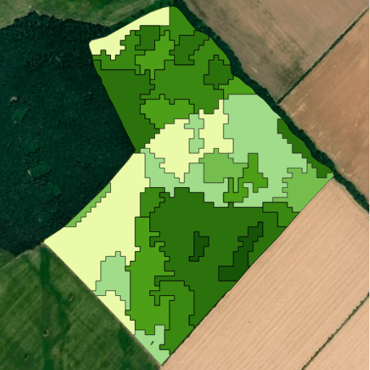
Fig. 1: Variable plot map
The CleverFarm app has the functionality to create maps for variable seeding and fertilization. In order to use this functionality you need to have a processed growth potential or use the biophysical variable monitoring service. You can read more about these services here:
and
Monitoring of biophysical parameters
Variable seeding
To create a variable seeding map, you will need to have the growth potential for the crop and a strategy for how to seed the plot. The basic strategies are to apply more seed to the stronger zone or to the weaker zone.
Example:
For cereals, a lower seeding density is recommended in zones with a higher production potential (best zone) and a higher density in zones with a lower potential. In zones with lower sowing densities, intensive propagation and a spontaneous increase in the number of producing individuals are expected.
The opposite strategy is recommended for maize or rape, for example. Apply a higher seeding density in the best zone.

Fig. 2: Variable seeding form
The resulting variable map is obtained in several steps. First you select a plot suitable for variable seeding, the growth potential for the selected crop and finally you select the seed and strategy. You can then generate and save the application map.
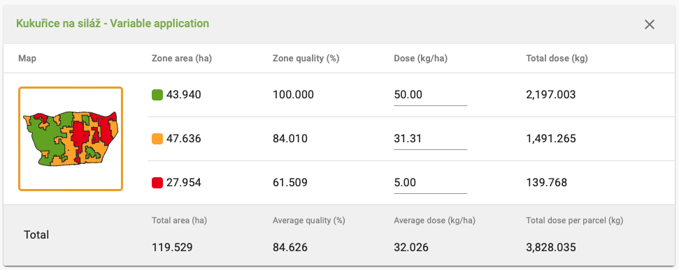
Fig. 3: Seed rate settings
Variable fertilisation
Fertilisation is usually divided into two types - balance (autumn) and production (spring).
Balance fertilisation is usually applied in autumn when the field is harvested. We assume that in the best zones the previous crop did well and therefore took more nutrients from the soil and needs to be replenished there, and conversely, in places where the yield was not high, there is no need to fertilise as much. The expected result of this type of variable fertilisation is to maintain a balanced nutrient balance on each plot. Hence the name balance fertilisation. It is mainly phosphorus and potassium that are supplemented.
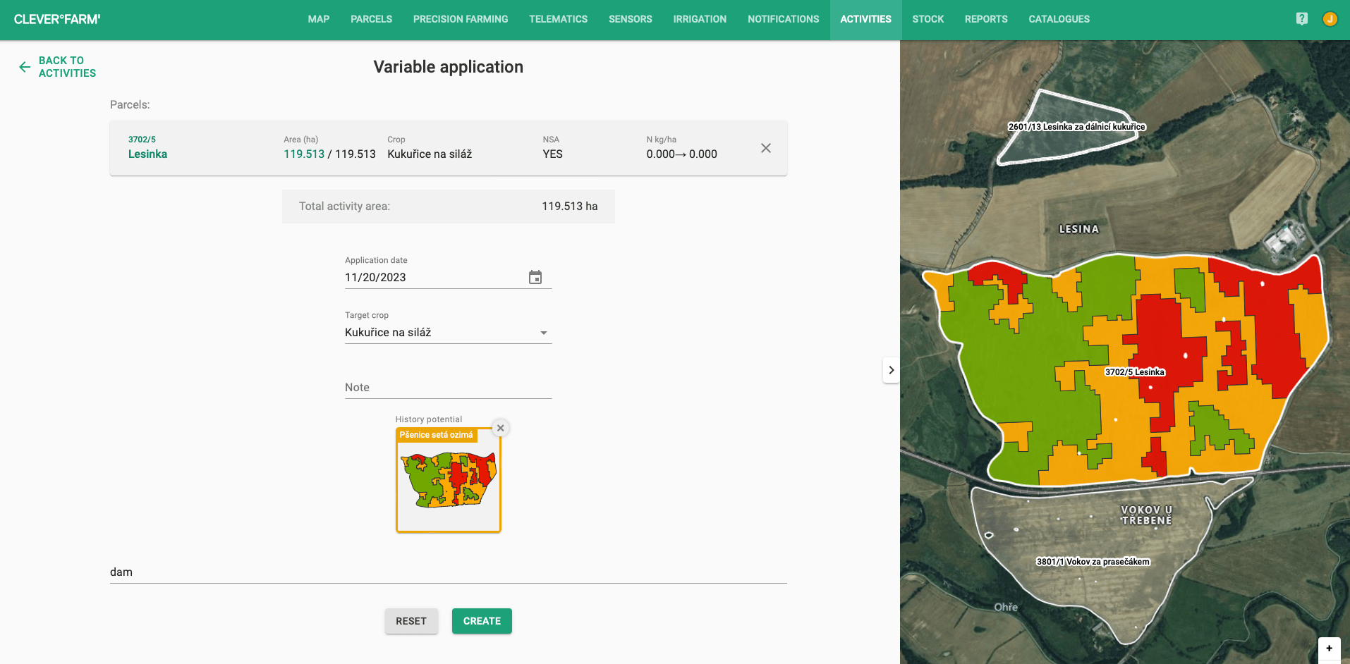
Fig. 4: Variable fertilisation formula
Based on the growth potential obtained from the satellite data, we can identify zones where more nutrients need to be added and conversely where fertilization is not needed as much. Variable fertilisation should make the whole process of post-harvest nutrient adjustment more efficient and bring considerable savings.
Production fertilisation takes place in the spring when the crop is already established in the field. Production fertiliser can be applied based on 3 inputs - current chlorophyll monitoring or leaf area index, or historical growth potential.
Difference between balance versus production fertilisation
The difference is in the data input - for balance fertilization, the input should only be the growth potential, whereas for production fertilization, the user can create a variable map from both the growth potential and the current chlorophyll monitoring or leaf area index.
Another major difference is that in balance fertilization, the strongest zones should receive the most fertilizer. In production fertilisation, however, the user can choose the strategy whether to apply more fertiliser to the good or bad zones.
How does this work in our application?
On plots where you have active growth potential or biomonitoring, you can create a new activity called Add Variable Fertilization. After entering the necessary parameters, you can select the fertilizer rates for each zone, as shown in Figure 5. After saving the parameters, a file will be ready for download, for now only in shp (ShapeFile) format.
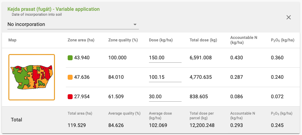
Fig. 5: Dose settings for individual zones